The quality and reliability of manufactured goods are highly dependent on the quality of component parts. If the quality of component parts is low, the quality and/or reliability of the end assembly will also be low. While some component parts are produced in house, many are procured from outside suppliers; the final quality is, therefore, highly dependent on suppliers.
In response to stiff competition, Ford Motor Company adopted procedural requirements for their suppliers in the early 1980s to insure the quality of incoming component parts. They demanded that all their suppliers show that their production processes were in a state of statistical control with a capability index greater than 1.5. Because Ford Motor Company bought such a large quantity of component parts from their suppliers, they were able to make this demand.
Smaller manufacturing companies may not have enough influence to make similar demands to their suppliers, and their component parts may come from several different suppliers and sub-contractors scattered across different countries and continents. However, by internal use of acceptance sampling procedures, they can be sure that the quality level of their incoming parts will be close to an agreed upon level. This chapter will illustrate how the \(\verb!AcceptanceSampling!\) and \(\verb!AQLSchemes!\) packages in R can be used both to create attribute sampling plans and sampling schemes and evaluate them.
When numerical measurements are made on the features of component parts received from a supplier, quantitative data results. On the other hand, when only qualitative characteristics can be observed, attribute data results. If only attribute data is available, incoming parts can be classified as either conforming/nonconforming, non-defective/defective, pass/fail, or present/absent etc. Attribute data also results from inspection data (such as inspection of billing records), or the evaluation of the results of maintenance operations or administrative procedures. Non conformance in these areas is also costly. Errors in billing records result in delayed payments and extra work to correct and resend the invoices. Non conformance in maintenance or administrative procedures, result in rework and less efficient operations.
A lot or Batch is defined as “a definite quantity of a product or material accumulated under conditions that are considered uniform for sampling purposes” (ASQ-Statistics 1996) . The only way that a company can be sure that every item in an incoming lot of components from a supplier, or every one of their own records or results of administrative work completed, meets the accepted standard is through 100% inspection of every item in the lot. However, this may require more effort than necessary, and if the inspection is destructive or damaging, this approach cannot be used.
Alternatively, a sampling plan can be used. When using a sampling plan, only a random sample of the items in a lot is inspected. When the number of nonconforming items discovered in the sample of inspected components is too high, the lot is returned to the supplier (just as a customer would return a defective product to the store). When inspecting the records of administrative work completed, and the number of nonconforming records or nonconforming operations are too high in a lot or period of time, every item in that period may be inspected and the work redone if nonconforming. On the other hand, if the number of nonconforming items discovered in the sample is low, the lot is accepted without further concern.
Although a small manufacturing company may not be able to enforce procedural requirements upon their suppliers, the use of an acceptance sampling plan will motivate suppliers to meet the agreed upon acceptance quality level or improve their processes so that it can be met. Otherwise, they will have to accept returned lots which will be costly.
When inspecting only a random sample from a lot, there is always a non-zero probability that there are nonconforming items in the lot even when there are no nonconforming items discovered in the sample. However, if the customer and supplier can agree on the maximum proportion nonconforming items that may be allowed in a lot, then an attribute acceptance sampling plan can be used successfully to reject lots with proportion nonconforming above this level. The sampling plan can both maximize the probability of rejecting lots with a higher proportion nonconforming than the agreed upon level (benefit to the customer), and it can maximize the probability of accepting lots that have the proportion nonconforming at or below the agreed upon level (benefit to the supplier).
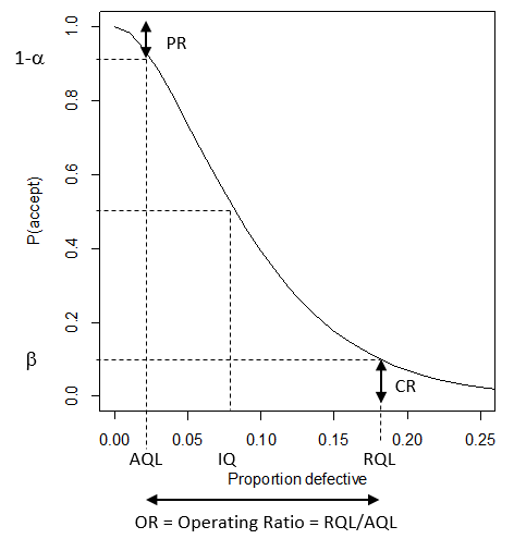
For a lot of \(N\) components, an attribute sampling plan consists of the number of items to be sampled, \(n\) , and the acceptance number or maximum number of nonconforming items, \(c\) , that can be discovered in the sample and still allow the lot to be accepted. The probability of accepting lots with varying proportions of nonconforming or defective items using an attribute acceptance sampling plan can be represented graphically by the OC (or Operating Characteristic) curve shown in Figure 2.1.
In this figure the AQL (Acceptance Quality Level) represents the agreed upon maximum proportion of nonconforming components in a lot. \(1-\alpha\) represents the probability of accepting a lot with the AQL proportion nonconforming, and the PR= \(\alpha\) is the producer’s risk or probability that a lot with AQL proportion nonconforming is rejected. The IQ is the indifference quality level where 50% of the lots are rejected, and RQL is the rejectable quality level where there is only a small probability, \(\beta\) , of being accepted. The customer should decide on the RQL. CR= \(\beta\) is the customer’s risk.
Figure 2.1 Operating Characteristic Curve
From the customer’s point of view, a steeper OC curve with a smaller operating ratio (or ratio of the RQL to the AQL) is preferable. In this case, the probability of accepting any lot with greater than the AQL proportion nonconforming is reduced. To prevent rejected lots, the supplier will be motivated to send lots with the proportion nonconforming less than the AQL. The ideal OC curve is shown in Figure 2.2. It would result when 100% inspection is used or \(n=N\) and \(c\) =AQL \(\times N\) . In this case, all lots with a proportion nonconforming (or defective) less than the AQL are accepted, and all lots with the proportion nonconforming greater than the AQL are rejected. As the fraction items sampled ( \(n/N\) ) in a sampling plan increases, the OC curve for that plan will approach the curve for the ideal case.
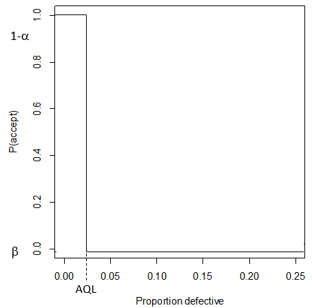
Figure 2.2 Ideal Operating Characteristic Curve for a Customer
Experience with sampling plans has led to the standard values of \(\alpha\) =PR=0.05 and \(\beta\) =CR=0.10 (Schilling and Neubauer 2017) . This will result in one lot in 20 rejected when proportion nonconforming is at the AQL, and only one lot in 10 accepted when the proportion nonconforming is at the RQL. When \(\beta\) =0.10, the RQL is usually referred to as the LTPD or Lot Tolerance Percent Defective. While \(\alpha=.05\) and \(\beta=0.10\) are common, other values can be specified. For example, if nonconforming items are costly then it may be desirable to use a \(\beta\) less than 0.10, and if rejecting lots that have the AQL proportion nonconforming is costly, it may be desirable to use \(\alpha\) less than 0.05.
In a single sampling plan, as described in the last section, all \(n\) sample units are collected before inspection or testing starts. Single sampling plans specify the number of items to be sampled, \(n\) , and the acceptance number, \(c\) . Single sampling plans can be obtained from published tables such as MIL-STD-105E, ANSI/ASQ Standard Z1.4, ASTM International Standard E2234, and ISO Standard 2859. Plans in these published tables are indexed by the lot size and AQL. The tables are most useful for the case when a purchaser buys a continuing stream of lots or batches of components, and the purchaser and seller agree to use the tables. More about these published sampling plans will be discussed in Section 2.6.
Custom derived sampling plans can be constructed for inspecting isolated lots or batches. Analytic procedures have been developed for determining the sample size, \(n\) , and the acceptance number, \(c\) , such that the probability of accepting a lot with the AQL proportion nonconforming will be as close as possible to \(1-\alpha\) , and the probability of accepting a lot with RQL proportion nonconforming will be as close as possible to \(\beta\) . These analytic procedures are available in the \(\verb!find.plan()!\) function in the R package \(\verb!AcceptanceSampling!\) that can be used for finding single sampling plans.
As an example of this function, consider finding a sampling plan where the AQL=0.05, \(\alpha\) =.05, RQL = 0.15, and \(\beta\) =0.20 for a lot of 500 items. For a plan where the sample size is \(n\) and the acceptance number is \(c\) , the probability of accepting a lot of \(N\) =500 with \(D\) nonconforming or defective items is given by the cumulative Hypergeometric distribution, i.e., \[\begin Pr(accept)=\sum_^\frac<\left(\begin D\\i \end\right) \left(\begin N-D\\n-i \end\right)> <\left(\begin N\\n \end\right)>. \tag \end\]
The \(\verb!find.plan!\) function attempts to find \(n\) and \(c\) so that the probability of accepting when \(D=0.05\times N\) is as close to 1-0.05=.95 as possible, and the probability of accepting when \(D=0.15\times N\) is as close to 0.20 as possible. The first statement in the R code below loads the \(\verb!AcceptanceSampling!\) package. The next statement is the call to \(\verb!find.plan!\) . The first argument in the call, \(\verb!PRP=c(0.05,0.95)!\) , specifies the producer risk point (AQL, 1- \(\alpha\) ); the second argument specifies the consumer risk point (RQL, \(\beta\) ); the next argument, \(\verb!type="hypergeom"!\) , specifies that the probability distribution is the hypergeometric; and the last argument, \(\verb!N=500!\) , specifies the lot size.
library(AcceptanceSampling) find.plan(PRP=c(0.05,0.95),CRP=c(0.15,0.20),type="hypergeom",N=500)In the output below we see that the sample size should be \(n\) =51 and the acceptance number \(c=5\) .
## $n ## [1] 51 ## ## $c ## [1] 5 ## ## $r ## [1] 6The following code produces the OC curve for this plan that is shown in Figure 2.3.
library(AcceptanceSampling) planOC2c(51,5,type="hypergeom", N=500, pd=seq(0,.25,.01)) plot(plan, type='l') grid()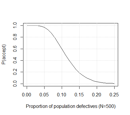
Figure 2.3 Operating Characteristic Curve for the plan with \(N=500\) , \(n=51\) , \(c=5\)
The code below shows how close the producer and consumer risk points for this plan are to the requirement.
library(AcceptanceSampling) assess(OC2c(51,5), PRP=c(0.05, 0.95), CRP=c(0.15,0.20)) Acceptance Sampling Plan (binomial) Sample 1 Sample size(s) 51 Acc. Number(s) 5 Rej. Number(s) 6 Plan CANNOT meet desired risk point(s): Quality RP P(accept) Plan P(accept) PRP 0.05 0.95 0.9589318 CRP 0.15 0.20 0.2032661The output shows the actual probability of acceptance at AQL is 0.9589 and the probability of acceptance at RQL is 0.2032.
To make the OC curve steeper and closer to the customer’s ideal, the required RQL can be made closer to the AQL. For example in the R code below, the RQL is reduced from 0.15 to 0.08. As a result, the \(\verb!find.plan!\) function finds a plan with a much higher sample size \(n=226\) (nearly 50% of the lot size \(N = 500\) ), and acceptance number \(c=15\) .
library(AcceptanceSampling) find.plan(PRP=c(0.05,0.95),CRP=c(0.08,0.20),type="hypergeom",N=500) $n [1] 226 $c [1] 15 $r [1] 16The OC curve for this plan is shown in Figure 2.4, and it is steeper with a reduced operating ratio. The disadvantage to this plan over the original ( \(n\) =51, \(c\) =5) plan is the increased sample size \(n\) =226. The next section discusses double and multiple sampling plans that can produce a steep OC curve with a smaller average sample size than required by a single sample plan.
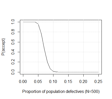
Figure 2.4 Operating Characteristic Curve for the plan with \(N=500\) , \(n=226\) , \(c=15\)
The aim of double sampling plans is to reduce the average sample size and still have the same producer and customer risk points. A double sampling plan consists of \(n_1\) , \(c_1\) , and \(r_1\) which are the sample size, acceptance, and rejection numbers for the first sample; \(n_2\) , \(c_2\) , and \(r_2\) , which are the sample size, acceptance number, and rejection number for the second sample.
A double sampling plan consists of taking a first sample of size \(n_1\) . If there are \(c_1\) or less nonconforming in the sample, the lot is accepted. If there are \(r_1\) nonconforming or more in the sample, the lot is rejected (where \(r_1\ge c_1+2\) ). If the number nonconforming in the first sample is between \(c_1+1\) and \(r_1-1\) , a second sample of size \(n_2\) is taken. If the sum of the number of nonconforming in the first and second samples is less than or equal to \(c_2\) , the lot is accepted. Otherwise, the lot is rejected. Although there is no function in the \(\verb!AcceptanceSampling!\) package in R for finding double sampling plans, the \(\verb!assess!\) function and the \(\verb!OC2c!\) function can be used to evaluate a double sampling plan, and the \(\verb!AQLSchemes!\) package can retrieve double sampling plans from the ANSI/ASQ Z1.4 Standard.
Consider the following example shown by (Schilling and Neubauer 2017) . If a single sampling plan that has \(n=134\) , and \(c=3\) is used for a lot of \(N=1000\) , it will have a steep OC curve with a low operating ratio. The R code below shows that there is at least a 96% chance of accepting a lot with 1% or less nonconforming, and less than an 8% chance of accepting a lot with 5% or more nonconforming.
library(AcceptanceSampling) plnsOC2c(n=134,c=3,type="hypergeom", N=1000,pd=seq(0,.20,.01)) assess(plns,PRP=c(.01,.95),CRP=c(.05,.10)) Acceptance Sampling Plan (hypergeom) Sample 1 Sample size(s) 134 Acc. Number(s) 3 Rej. Number(s) 4 Plan CAN meet desired risk point(s): Quality RP P(accept) Plan P(accept) PRP 0.01 0.95 0.96615674 CRP 0.05 0.10 0.07785287However, the sample size ( \(n\) =134) is large, over 13% of the lot size. If a double sampling plan with \(n_1=88\) , \(c_1=1\) , \(r_1=4\) , and \(n_2=88\) , \(c_2=4\) , \(r_2=5\) is used instead, virtually the same customer risk will result, and slightly less risk for the producer. This is illustrated by the R code below.
library(AcceptanceSampling) pln3OC2c(n=c(88,88),c=c(1,4),r=c(4,5),type="hypergeom",N=1000,pd=seq(0,.20,.01)) assess(pln3,PRP=c(.01,.95),CRP=c(.05,.10)) Acceptance Sampling Plan (hypergeom) Sample 1 Sample 2 Sample size(s) 88 88 Acc. Number(s) 1 4 Rej. Number(s) 4 5 Plan CAN meet desired risk point(s): Quality RP P(accept) Plan P(accept) PRP 0.01 0.95 0.9805612 CRP 0.05 0.10 0.0776524In the code above, the first argument to the \(\verb!OC2c!\) function, \(\verb!n=c(88,88)!\) specifies \(n_1\) and \(n_2\) for the double sampling plan. The second argument \(\verb!c=c(1,4)!\) specifies \(c_1\) and \(c_2\) , and the third argument \(\verb!r=c(4,5)!\) specifies \(r_1\) and \(r_2\) . Notice that \(r_2=c_2+1\) because a decision must be made after the second sample.
The sample size for a double sampling plan will vary between \(n_1\) and \(n_1+n_2\) depending on whether the lot is accepted or rejected after the first sample. The probability of accepting or rejecting after the first sample depends upon the number of nonconforming items in the lot, therefore the average sample number (ASN) for the double sampling plan will be:
where \(x_1\) is the number of nonconforming items found in the first sample.
The R code below creates Figure 2.5 that compares the sample size for the single sampling plan with the average sample for a double sampling plan at various proportions nonconforming or defective in the lot.
library(AcceptanceSampling) D=seq(0,200,5) #Number nonconforming in the lot of 1000 pd/1000 #Proportion nonconforming in the lot of 1000 OC1phyper(1, m=D, n=1000-D, k=88, lower.tail=TRUE) #Probability of accepting after the first sample R1phyper(3, m=D, n=1000-D, k=88, lower.tail=FALSE) #Probability of rejecting after the first sample P+R1 ASN=88+88*(1-P) plot(pd,ASN,type='l',ylim=c(5,150),xlab="Proportion nonconforming in the lot") abline(134,0,lty=2) text(.10,142,'single sample n=134') text(.10,70,'double sample n=(88,88)') grid()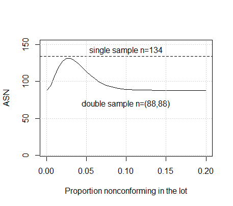
Figure 2.5 Comparison of Sample sizes for Single and Double Sampling Plan
From this figure it can be seen that the average combined sample size for the double sampling plan is uniformly less than the equivalent single sampling plan. The average sample size for the double sampling plan saves most when the proportion nonconforming in the lot is less than the AQL or greater than the RQL.
The disadvantage of a double sampling plan is that they are very difficult or impossible to apply when the testing or inspection takes a long time or must be performed off site. For example, food safety and microbiological tests may take 2 to 3 days for obtaining the results.
Multiple sampling plans extend the logic of double sampling plans, by further reducing the average sample size. Multiple sampling plans can be presented in tabular form as shown in Table 2.1
Table 2.1: A Multiple Sampling Plan
| Sample | Sample Size | Cum. Samp. Size | Acc. Number | Rej. Number |
|---|---|---|---|---|
| 1 | \(n_1\) | \(n_1\) | \(c_1\) | \(r_1\) |
| 2 | \(n_2\) | \(n_1+n_2\) | \(c_2\) | \(r_2\) |
| \(\vdots\) | \(\vdots\) | \(\vdots\) | \(\vdots\) | \(\vdots\) |
| k | \(n_k\) | \(n_1+n_2+\ldots+n_k\) | \(c_k\) | \(r_k=c_k+1\) |
If \(x_1 \leq c_1\) (where \(x_1\) is the number of nonconforming items found in the first sample) the lot is accepted. If \(x_1 \ge r_1\) the lot is rejected, and if \(c_1
A multiple sampling plan with a similar OC curve as a double sampling plan will have an even lower ASN curve than the double sampling plan. The multiple sampling plan shown in Table 2.2, has an OC curve that is very similar to the single ( \(n\) =134, \(c\) =3) and the double sampling plan ( \(n_1\) =88, \(n_2\) =88, \(c_1\) =1, \(c_2\) =4, \(r_1\) =4, \(r_2\) =5) presented above. Figure 2.6 shows a comparison of their OC curves magnifying on the region where these curves are steepest. It can be seen that within the region of the AQL=0.01 and the RQL = 0.05, these OC curves are very similar. The ASN curve for the multiple sampling plan can be shown to fall below the ASN curve for the double sampling plan shown in Figure 2.5.
Although the \(\verb!AcceptanceSampling!\) package does not have a function for creating double or multiple sampling plans for attributes, the ANSI/ASQ Z1.4 tables discussed in Section 2.7.2 present single, double, and multiple sampling plans with matched OC curves. The single, double, and multiple sampling plans in these tables can be accessed with the \(\verb!AQLSchemes!\) package or with the sqc online calculator. The tables also present the OC curves and ASN curves for these plans, but the same the OC and ASN curves can be obtained from the \(\verb!AQLSchemes!\) package as well.
Table 2.2: A Multiple Sampling Plan with k=6
| Sample | Sample Size | Cum. Samp. Size | Acc. Number | Rej. Number |
|---|---|---|---|---|
| 1 | 46 | 46 | 0 | 3 |
| 2 | 46 | 92 | 1 | 3 |
| 3 | 46 | 138 | 2 | 4 |
| 4 | 46 | 184 | 3 | 5 |
| 5 | 46 | 230 | 4 | 6 |
| 6 | 46 | 276 | 6 | 7 |
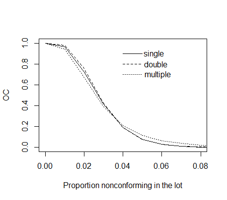
Figure 2.6 Comparison of OC Curves
The \(\verb!OC2c!\) , and \(\verb!assess!\) functions in the \(\verb!AcceptanceSampling!\) package, and the R \(\verb!plot!\) function can be used to evaluate the properties of a multiple sampling plan as shown in the R code below.
library(AcceptanceSampling) pln4OC2c(n=c(46,46,46,46,46,46),c=c(0,1,2,3,4,6), r=c(3,3,4,5,6,7), + type="hypergeom",N=1000,pd=seq(0,.20,.01)) assess(pln4,PRP=c(.01,.95),CRP=c(.05,.10)) plot(pln4,type='l') summary(pln4,full=TRUE)In summary, a sampling plan with a steeper OC curve is preferable. It benefits the customer by reducing the chances of accepting lots containing a proportion nonconforming higher than the AQL, and it motivates the supplier to send lots with a proportion nonconforming less than the AQL to avoid having lots returned. It also benefits a supplier of good quality because the probability of having a lot rejected that contains a proportion nonconforming less than the AQL is reduced.
Single sampling plans are the easiest to administer; however, the disadvantage of a single sampling plan with a steep OC curve is the additional cost of increased sampling. An equivalently steep OC curve can result from a double or multiple sampling plan with a lower average sample number (ASN). This is the advantage of double and multiple sampling plans. The disadvantage of double or multiple sampling plans is the increased bookkeeping and additional decisions that must be made.
When rectification sampling is used, every nonconforming item found in the sample is replaced with a conforming item. Further, if the lot is rejected, the remaining items in the lot are also inspected, and any additional nonconforming items found are replaced by conforming items. In that way every rejected lot will be 100% inspected and all nonconforming items replaced with conforming items. This results in two different sampling plans (sample inspection or 100% inspection). Which one is used for a particular lot depends whether the lot is rejected based on the first sample. By use of rectification inspection, the average percent nonconforming in lots leaving the inspection station can be guaranteed to be below a certain level. This type of inspection is often used where component parts or records are produced and inspected in-house.
Assuming that an ongoing stream of lots is being inspected, the OC or probability that a lot is accepted by a single sampling plan for attributes is given by the Binomial Distribution \[\begin P_a=\sum_^ \left(\begin n\\i \end\right) p^i(1-p)^ \tag \end\]
where \(n\) is the sample size, \(c\) is the acceptance number and \(p\) is the probability of a nonconforming item being produced in the supplier’s process. The average outgoing quality AOQ is given by \[\begin AOQ = \frac \tag \end\] where \(N\) is the lot size. The AOQ is a function of the probability of a nonconforming being produced in the supplier’s process. The AOQL or average outgoing quality limit is the maximum value of AOQ. For a lot of size \(N =\) 2000, and a single sampling plan consisting of \(n =\) 50, and \(c =\) 2, the R code shown below, calculates the AOQ and plots it versus \(p\) . The plot is shown in Figure 2.7.
pseq(.01,.15,.01) N2000 n50 c2 Papbinom(c,n,p,lower.tail=TRUE) AOQ<-(Pa*p*(N-n))/N plot(p,AOQ,type='b',xlab='Probability of nonconforming') lines(c(.02,.08),c(.02639,.02639),lty=2) text(.088,.02639,"AOQL")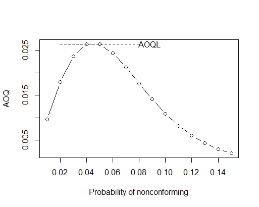
Figure 2.7 AOQ Curve and AOQL
From this figure, it can be seen that rectification inspection could guarantee that the average proportion nonconforming in a lot leaving the inspection station is about 0.027.
For a single sampling plan with rectification, the number of items inspected is either \(n\) or \(N\) , and the average total inspection (ATI) required is \[\begin ATI = n + (1-P_a)(N-n). \tag \end\]
If rectification is used with a double sampling plan, \[\begin \begin ASN&=n_1(P_+P_)+n_2(1-P_-P_)\\ \\ ATI&=n_1P_+(n_1+n_2)P_+N(1-P_-P_) \end \tag \end\]
where \(n_1\) is sample size for the first sample, \(n_2\) is the sample size for the second sample, \(P_\) is the probability of accepting on the first sample, and \(P_\) is the probability of accepting on the second sample, which is given by \(\sum_^P(x_1=i)P(x_2\leq c_2-x_1)\) where \(x_1\) is the number nonconforming on the first sample and \(x_2\) is the number nonconforming on the second sample.
Dodge and Romig developed tables for rectification plans in the late 1920s and early 1930s at the Bell Telephone Laboratories. Their tables were first published in the Bell System Technical Journal and later in book form (Dodge and Romig 1959) . They provided both single and double sampling for attributes.
There are two sets of plans. One set minimized the ATI for various values of the LTPD. The other set of tables minimize the ATI for a specified level of AOQL protection. The LTPD based tables are useful when you want to specify an LTPD protection on each lot inspected. The AOQL based plans are useful to guarantee the outgoing quality levels regardless of the quality coming to the inspection station. The tables for each set of plans require that the supplier’s process average percent nonconforming be known. If this is not known, it can be entered as the highest level shown in the table to get a conservative plan.
The LTPD based plans provide more protection on individual lots and therefore require higher sample sizes than the AOQL based plans. While this book by does not contain the Dodge Romig tables, they are available in the book by (Montgomery 2013) and the online sample size calculator at https://www.sqconline.com/ will provide the single sample plans for both AOQL and LTPD protection (note: sqconline offers free access for educational purposes).
When used by a supply process within the same company as the customer, a more recent and better way of insuring that the average proportion nonconforming is low is to use the quality management techniques and statistical process control techniques advocated in MIL-STD-1916. Statistical process control techniques will be discussed in Chapters 4, 5, and 6.
Acceptance sampling plans are most effectively used for inspecting isolated lots. The OC curves for these plans are based on the Hypergeometric distribution and are called Type A OC Curves in the literature. On the other hand, when a customer company expects to receive ongoing shipments of lots from a trusted supplier, instead of one isolated lot, it is better to base the OC curve on the Binomial Distribution, and it is better to use a scheme of acceptance sampling plans (rather than one plan) to inspect the incoming stream of lots.
When a sampling scheme is utilized, there is more than one sampling plan and switching rules to dictate which sampling plan should be used at a particular time. The switching rules are based on previous samples. In a sense, the Dodge-Romig Rectification plans represent a scheme. Either a sampling inspection plan or 100% inspection is used, based on results of the sample. A sampling scheme where the switching rules are based on the result of sampling the previous lot will be described in the next section.
When basing the OC curve on the Binomial Distribution, the OC or probability of acceptance is given by:
where \(n\) is the sample size taken from each lot, \(c\) is the acceptance number, and \(p\) is the probability of a nonconforming item being produced in the suppliers process. In the literature an OC curve based on the Binomial Distribution is called a Type B OC Curve.
(Romboski 1969) proposed a straightforward sampling scheme called the quick switching scheme QSS-1. His plan proceeds as follows. There are two acceptance sampling plans. One is called the normal inspection plan consisting of sample size \(n\) and acceptance number \(c_N\) , the second is called the tightened inspection plan consisting of the same sample size \(n\) , but a reduced acceptance number \(c_T\) . The following switching rules are used:
This plan can be diagrammed simply as shown in Figure 2.8.
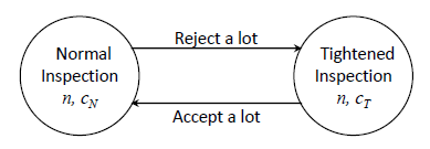
Figure 2.8 Romboski’s QSS-1 Quick Switching System
For the case where \(n=\) 20, \(c_N=\) 1, and \(c_T=\) 0, Figure 2.9 compares the OC curves for the normal and tightened plans. Using the normal plan will benefit the supplier with at least a 0.94 probability of accepting lots with an average of 2% nonconforming or less. However, this plan is less than ideal for the customer who will have less than a 0.50 probability of rejecting a lot with 8% nonconforming. Using the tightened inspection plan, the customer is better protected with a more than 0.80 probability of rejecting a lot with 8% nonconforming. Nevertheless, the tightened plan OC curve is very steep in the acceptance quality range, and there is greater than a 0.32 probability of rejecting a lot with only 2% nonconforming. This would be unacceptable to most suppliers.
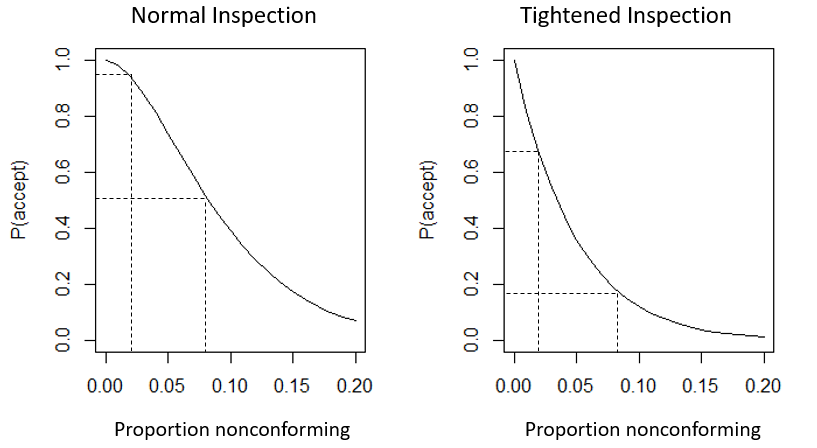
Figure 2.9 Comparison of Normal and Tightend Plan OC Curves
Using the switching rules, the quick switching scheme results in a compromise between the normal inspection plan that favors the supplier and the tightened inspection plan that benefits the customer. The OC curve for the scheme will be closer to the ideal OC curve shown in Figure 2.2 without increasing the sample size.
The scheme OC curve will have a shoulder where there is a high probability of accepting lots with a low percent nonconforming, like the OC curve for the normal inspection plan. This benefits a supplier of good quality. In addition, it will drop steeply to the right of the AQL, like the OC curve for the tightened plan. This benefits the customer.
The scheme can be viewed as a two state Markov chain with the two states being normal inspection and tightened inspection. Based on this fact, (Romboski 1969) determined that the OC or probability of acceptance of a lot by the scheme (or combination of the two plans) was given by
where \(P_N\) is the probability of accepting under normal inspection, that is given by the Binomial Probability Distribution as:
and \(p\) is the probability of a nonconforming item being produced in the suppliers process. \(P_T\) is the probability of accepting under tightened inspection, and is given by the Binomial Probability Distribution as
For the quick switching scheme with \(n\) =20, \(c_N\) =1, and \(c_T\) =0, the R code below uses Equations (2.8) to (2.10) to calculate the OC curves for the scheme, normal, and tightened inspection, and then creates a graph shown in Figure 2.10 to compare them.
# Comparison of Normal, Tightened, and QSS-1 OC Curves pdseq(0,.20,.005) PN=pbinom(1,20,pd) PT=pbinom(0,20,pd) Pa/((1-PN)+PT) plot(pd,Pa,type='l',lty=1,xlim=c(0,.2),xlab='Probability of a nonconforming',ylab="OC") lines(pd,PN,type='l',lty=2) lines(pd,PT,type='l',lty=3) lines(c(.10,.125),c(.9,.9),lty=1) lines(c(.10,.125),c(.8,.8),lty=2) lines(c(.10,.125),c(.7,.7),lty=3) text(.15,.9,'Scheme') text(.15,.8,'Normal') text(.15,.7,'Tightened')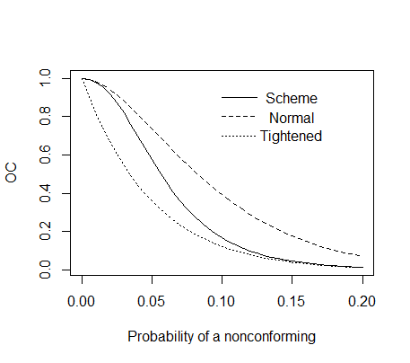
Figure 2.10 Comparison of Normal, Tightend, and Scheme OC Curves
In this figure it can be seen that the OC curve for the QSS-1 scheme is a compromise between the OC curves for the normal and tightened sampling plans, but the sample size, \(n =\) 20, is the same for the scheme as it is for either of the two sampling plans.
In addition to the QSS-1 scheme resulting in an OC curve that is closer to the ideal curve shown in Figure 2.2 without increasing the sample size \(n\) , there is one additional benefit. If a supplier consistently supplies lots where the proportion nonconforming is greater than the level that has a high probability of acceptance, there is a increased chance that the sampling will be conducted with the tightened plan, and this will result in a lower probability of acceptance. If all rejected lots are returned to the supplier, this will be costly for the supplier and will be a motivation for the supplier to reduce the proportion nonconforming. Therefore, although small customers may not be able to require procedural requirements for their suppliers to improve quality levels (as Ford Motor Company did in the early 1980’s), the use of a sampling scheme to inspect incoming lots will motivate suppliers to improve quality levels themselves.
The United States Military developed sampling inspection schemes as part of the World War II effort. They needed a system that did not require 100% inspection of munitions. In subsequent years improvements led to MIL-STD-105A, B, …, E. This was a very popular system worldwide, and it was used for government and non-government contracts. The schemes in MIL-STD were based on the AQL and lot size and are intended to be applied to a stream of lots. They include sampling plans for normal, tightened, reduced sampling, and associated switching rules. Single sampling plans, double sampling plans and multiple sampling plans with equivalent OC curves are available for each lot size - AQL combination.
However, in 1995 the Army discontinued supporting the MIL-STD-105E. Civilian standards-writing organizations such as the American Standards Institute (ANSI), the International Standards Organization (ISO) and others have developed their own derivatives of the MIL-STD-105E system. The ANSI/ASQ Standard Z1.4 is the American national standard derived from MIL-STD-105E. It incorporates minor changes, none of which involved the central tables. It is recommended by the Department of Defense as a replacement and is best used for domestic contracts and in house-use. The complete document is available for purchase online at https://asq.org/quality-press/display-item?item=T964E. The textbook by (Christensen, Betz, and Stein 2013) only includes the ANSI/ASQ Z1.4 tables for normal inspection. The R package \(\verb!AQLSchemes!\) as well as the sqc online calculator contains functions that will retrieve the normal, tightened, or reduced single and double sampling plans from the ANSI/ASQ Z1.4 Standard. The rules for switching between Normal, tightened, and reduced sampling using ANSI/ASQ Z1.4 standard are shown in Figure 2.11. Utilizing the plans and switching rules will result in an OC curve closer to the ideal, and will motivate the suppliers to provide lots with the proportion nonconforming at or below the agreed upon AQL.
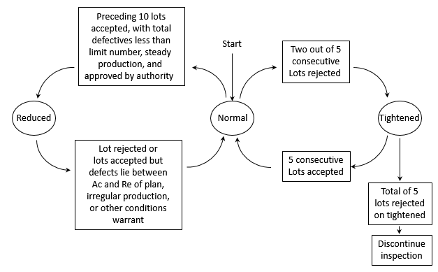
Figure 2.11 Switching rules for ANSI/ASQ Z1.4 (Reproduced from (Schilling and Neubauer 2017) )
The international standard, ISO 2859-1, incorporates modifications to the original MIL-STD-105 concepts to reflect changes in the state of the art, and it is recommended for use in international trade. Again, proper use of the plans requires adherence to the switching rules which are shown in Figure 2.12. When this is done, the producer receives protection against having lots rejected when the percent nonconforming is less than the stated AQL. The customer is also protected against accepting lots with a percent nonconforming higher than the AQL. When the rules are not followed, these benefits are lost. The benefit of smaller sample sizes afforded to the customer by the reduced plan, when quality is good, is also lost when the switching rules are not followed.
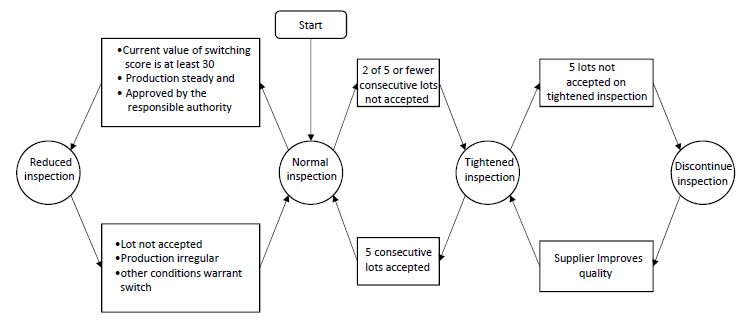
Figure 2.12 Switching rules for ISO 2859-1
The calculation of the switching score in Figure 2.12 is initiated at the start of normal inspection unless otherwise specified by a responsible authority. The switching score is set to zero at the start and is updated following the inspection of each subsequent lot on original normal inspection.
a) Single sampling plans:
b) Double or multiple sampling plans:
To use the tables from ANSI/ASQ Z1.4 or ISO 2859-1, a code letter is determined from a table, based on the lot size and inspection level. Next, a decision is made whether to use single, double, or multiple sampling, and whether to use normal, tightened, or reduced inspection. Finally, the sample size(s) and acceptance-rejection number(s) are obtained from the tables. The online NIST Engineering Statistics Handbook ( - http://www.itl.nist.gov/div898/handbook/ Section 6.2.3.1) shows an example of how this is done using the MIL-STD 105E-ANSI/ASQ Z1.4 tables for normal inspection.
The section of R code below shows how the single sampling plan for this same situation can be retrieved using the \(\verb!AASingle()!\) function in the R package \(\verb!AQLSchemes!\) . The function call \(\verb!AASingle('Normal')!\) shown below specifies that the normal sampling plan is desired. When this function call is executed, the function interactively queries the user to determine the inspection level, the lot size, and the AQL. The result is a sampling plan with \(n\) =125, with an acceptance number \(c\) =5, and a rejection number \(r\) =6 as shown in the section of code below.
> library(AQLSchemes) > planSAASingle('Normal') MIL-STD-105E ANSI/ASQ Z1.4 If the sample size exceeds the lot size carry out 100% inspection What is the Inspection Level? 1: S-1 2: S-2 3: S-3 4: S-4 5: I 6: II 7: III Selection: 6 What is the Lot Size? 1: 2-8 2: 9-15 3: 16-25 4: 26-50 5: 51-90 6: 91-150 7: 151-280 8: 281-500 9: 501-1200 10: 1201-3200 11: 3201-10,000 12: 10,001-35,000 13: 35,001-150,000 14: 150,001-500,000 15: 500,001 and over Selection: 10 What is the AQL in percent nonconforming per 100 items? 1: 0.010 2: 0.015 3: 0.025 4: 0.040 5: 0.065 6: 0.10 7: 0.15 8: 0.25 9: 0.40 10: 0.65 11: 1.0 12: 1.5 13: 2.5 14: 4.0 15: 6.5 16: 10 17: 15 18: 25 19: 40 20: 65 21: 100 22: 150 23: 250 24: 400 25: 650 26: 1000 Selection: 12 > planS n c r 1 125 5 6Executing the function call again with the option tightened (i.e., \(\verb!AASingle('Tightened')!\) and answering the queries the same as above results in the tightened plan with \(n\) =125, \(c\) =3, and \(r\) =4. The reduced sampling plan is obtained by executing the function \(\verb!AASingle('Reduced')!\) and answering the queries the same way. This results in a plan with less sampling required (i.e., \(n\) =50, \(c\) =2, and \(r\) =5). However, there is a gap between the acceptance number and the rejection number. Whenever the acceptance number is exceeded in a ANSI/ASQ Z1.4 plan for reduced inspection, but rejection number has not been reached (for example if the number of nonconformities in a sample of 50 were 4 in the last example) then the lot should be accepted, but normal inspection should be reinstated.
One of the modifications incorporated when developing the ISO 2859-1 international derivative of MIL-STD 105E was the elimination of gaps between the acceptance and rejection numbers. the ISO 2859-1 single sampling plan, for the lot size AQL and inspection level in the example above, are the same for the normal and tightened plans, but the reduced plan is \(n\) =50, \(c\) =3, and \(r\) =4 with no gap between the acceptance and rejection numbers.
To create an ANSI/ASQ Z1.4 double sampling plan for the same requirements as the example above using the \(\verb!AQLSchemes!\) package, use the \(\verb!AADouble()!\) function as shown in the example below.
> library(AQLSchemes) > planDAADouble('Normal') MIL-STD-105E ANSI/ASQ Z1.4 What is the Inspection Level? 1: S-1 2: S-2 3: S-3 4: S-4 5: I 6: II 7: III Selection: 6 What is the Lot Size? 1: 2-8 2: 9-15 3: 16-25 4: 26-50 5: 51-90 6: 91-150 7: 151-280 8: 281-500 9: 501-1200 10: 1201-3200 11: 3201-10,000 12: 10,001-35,000 13: 35,001-150,000 14: 150,001-500,000 15: 500,001 and over Selection: 10 What is the AQL in percent nonconforming per 100 items? 1: 0.010 2: 0.015 3: 0.025 4: 0.040 5: 0.065 6: 0.10 7: 0.15 8: 0.25 9: 0.40 10: 0.65 11: 1.0 12: 1.5 13: 2.5 14: 4.0 15: 6.5 16: 10 17: 15 18: 25 19: 40 20: 65 21: 100 22: 150 23: 250 24: 400 25: 650 26: 1000 Selection: 12 > planD n c r first 80 2 5 second 80 6 7As can be seen in the output above, the sample sizes for the double sampling plan are 80, and 80. Accept after the first sample of 80 if there are 2 or less nonconforming, and reject if there are 5 or more nonconforming. If the number nonconforming in the first sample of 80 is 3 or 4, take a second sample of 80 and accept if the combined total of nonconforming items in the two samples is 6 or less, otherwise reject.
The OC curves are very similar for the single and double sampling plans, but not exactly the same. The OC curves for the single sampling plan ( \(n\) =125, \(c\) =5) and the double sampling plan created with the \(\verb!AASingle()!\) and \(\verb!AADouble()!\) functions were determined separately and are compared in Figure 2.16. This figure also compares the ASN curve for the double sampling plan to the constant sample size for the single sampling plan. This figure was created with the R-code shown below. In this code the \(\verb!OCASNZ4S()!\) and \(\verb!OCASNZ4D()!\) functions in the \(\verb!AQLSchemes!\) package were used to create the coordinates of the OC curves and the ASN curve for the double sampling plan. The result of these functions is a data frame with columns for the proportion defective (pd) the probability of acceptance (OC) and the average sample number (ASN). The statements OCS
library(AQLSchemes) par(mfcol=c(1,2)) Pncseq(0,.15,.01) SOCASNOCASNZ4S(planS,Pnc) DOCASNOCASNZ4D(planD,Pnc) OCS$OC OCD$OC ASND$ASN # plot OC Curves plot(Pnc,OCS,type='l', xlab='Proportion Nonconforming', ylab='OC', lty=1) lines(Pnc,OCD, type='l', lty=2,col=2) legend(.04,.95,c("S","D"),lty=c(1,2),col=c(1,2)) # ASN Curves plot(Pnc,ASND,type='l',ylab='ASN',lty=2,col=2,ylim=c(60,160)) lines(Pnc,rep(125,16),lty=1) par(mfcol=c(1,2))This figure shows that the OC curves for normal sampling with either the single or double sampling plan for the same inspection level, lot size, and AQL, are virtually equivalent. However, the double sampling plan provides slightly greater protection for the customer at intermediate levels of the proportion nonconforming. Another advantage of the double sampling plan is that the average sample size will be uniformly less than the single sampling plan.
To create ANSI/ASQ Z1.4 double sampling plans for tightened, or reduced plans use the function call \(\verb!AADouble('Tightened')!\) or \(\verb!AADouble('Reduced')!\) when the \(\verb!AQLSchemes!\) package is loaded. Similarly the normal tightened, or reduced multiple sampling plans for ANSI/ASQ Z1.4 can be recalled with the commands \(\verb!AAMultiple('Normal')!\) , \(\verb!AAMultiple('Tightened')!\) , and \(\verb!AAMultiple('Reduced')!\) .
The OC curve for a multiple sampling plan for the same inspection level, lot size, and AQL, will be virtually the same as the OC curves for the single and double sampling plans shown in Figure 2.16, and the ASN curve will be uniformly below the ASN curve for the double sampling plan. This will be the case for all ANSI/ASQ Z1.4 and ISO 2859-1 single double and multiple sampling plans that are matched for the same conditions.
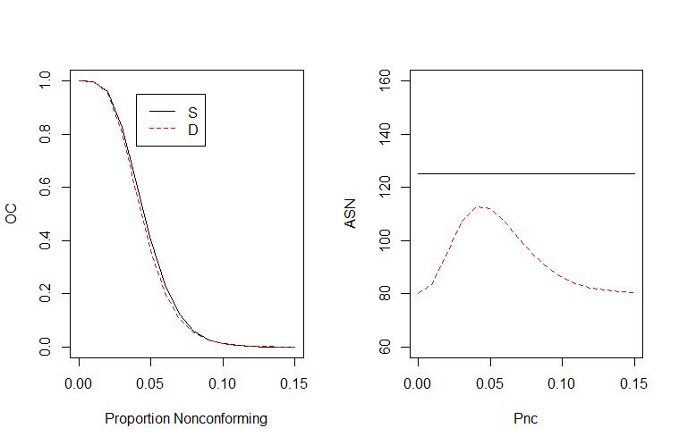
Figure 2.13 Comparison of OC and ASN Curves for ANSI/ASQ Z1.4 Single and Double Plans
(Stephens and Larson 1967) investigated the properties of MIL-STD-105E, which is also relevant to ANSI/ASQ Standard Z1.4, and the ISO 2859-1. When ignoring the reduced plan (the use of which requires authority approval) and considering only the normal-tightend system, the sampling scheme again can be viewed as a two state Markov chain with the two states being normal inspection and tightened inspection. They showed the OC or probability of accepting by this scheme is given by the following equation:
where \(P_N\) is the probability of accepting under normal inspection, \(P_T\) is the probability of accepting under tightened inspection, and
In addition, \(a/(a+b)\) is the steady state probability of being in the normal sampling state, and \(b/(a+b)\) is the steady state probability of being in the tightened sampling state. Therefore, the average sample number (ASN) for the normal-tightened scheme is given by the equation
To illustrate the benefit of using the ANSI/ASQ Standard Z1.4 sampling scheme for attribute sampling, consider the case of using a single sampling scheme for a continuing stream of lots with lot sizes between 151 and 280. The code letter is G. If the required AQL is 1.0 (or 1%), then the normal inspection plan is \(n =\) 50, with \(c =\) 1, and the tightened inspection plan is \(n =\) 80, with \(c =\) 1.
The R code below computes the OC curve and the ASN curve and plots them in Figure 2.14. Responses to the queries resulting from the commands \(\verb!AASingle('Normal')!\) and \(\verb!AASingle('Tightened')!\) were 6, 7, and 11.
# Comparison of Normal, Tightened, and Scheme OC and ASN Curves library(AQLSchemes) planSNAASingle('Normal') planSTAASingle('Tightened') par(mfcol=c(1,2)) Pncseq(0,.15,.002) SNOCASNOCASNZ4S(planSN,Pnc) STOCASNOCASNZ4S(planST,Pnc) PN$OC PT$OC ASNN$ASN ASNT$ASN a=(2-PN^4)/((1.0000000000001-PN)*(1.0000000000001-PN^4)) b=(1.0000000000001-PT^5)/((1.0000000000001-PT)*(PT^5)) PS<-(a*PN+b*PT)/(a+b) plot(Pnc,PS,type='l',lty=1,xlim=c(0,.1),xlab='Probability of nonconforming',ylab="OC",col=1) lines(Pnc,PN,type='l',lty=2,col=3) lines(Pnc,PT,type='l',lty=3,col=2) lines(c(.05,.06),c(.9,.9),lty=1,col=1) lines(c(.05,.06),c(.8,.8),lty=2,col=3) lines(c(.05,.06),c(.7,.7),lty=3,col=2) text(.08,.9,'Scheme',col=1) text(.08,.8,'Normal',col=3) text(.08,.7,'Tightened',col=2) # ASN for Scheme ASN<-(a/(a+b))*ASNN+(b/(a+b))*ASNT plot(Pnc,ASN,type='l',ylim=c(40,90),xlim=c(0,.025),xlab="Probability of nonconforming", ylab="ASN") lines(Pnc,ASNN,type='l',lty=2,col=3) lines(Pnc,ASNT,type='l',lty=3,col=2) par(mfcol=c(1,1))The left side of Figure 2.17 shows a comparison of the OC curves for this single sampling scheme that uses the switching rules with the individual, normal, and tightened plans. Again, the OC curve for the scheme is a compromise between the normal and tightened plan. The right side of the figure shows the ASN curve for the scheme.
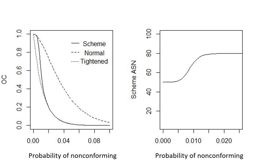
Figure 2.17 Comparison of Normal, Tightend, and Scheme OC Curves and ASN for Scheme
It can be seen from the figure that the OC curve for the scheme is very steep with an AQL (with 0.95 probability of acceptance) of about 0.005 or .5%, and an LTPD (with 0.10 probability of acceptance) of about 0.0285 or 2.85%. Notice the AQL is actually less than the required AQL of 1% used to find the sample sizes and acceptance numbers in the MIL-STD-105E or ANSI/ASQ Standard Z1.4 Tables. Therefore, whenever you find a normal, tightend, or reduced plan in the tables, you should check the OC curve (or a summary of the plan should be printed) to find the actual AQL and LTPD. To find a custom single sampling plan using the \(\verb!find.plan()!\) function in the \(\verb!AcceptanceSampling!\) package with an equivalent OC curve, with the producer risk point of (.005, .95) and customer risk point of (.0285, .10), would require a sample size \(n =\) 233.
It can be seen from the right side of the Figure 2.17 that the ASN for the scheme falls between \(n_N =\) 50 and \(n_T =\) 80. As the probability of a nonconforming in the lot increases beyond the LTPD, the scheme will remain in the tightened sampling plan with the sample size of 80. This is still less than half the sample size required by an equivalent single sampling plan.
For the same lot size and required AQL, the MIL-STD-105E tables also provide double and multiple sampling schemes with equivalent OC curves. The double sampling scheme for this example is shown in Table 2.3 and uses the same switching rules shown in Figure 2.11. The multiple sampling plan is shown in Table 2.4, and again uses the same switching rules.
The double sampling scheme will have a uniformly smaller ASN than the single sampling scheme, shown in Figure 2.14, and the multiple sampling scheme will have a uniformly smaller ASN than the double sampling scheme. The double and multiple sampling schemes will require more bookkeeping to administer, but they will result in reduced sampling with the same protection for producer and supplier.
Table 2.3: The ANSI/ASQ Z1.4 Double Sampling Plan
| Sample | Sample Size | Cum. Samp. Size | Acc. Number | Rej. Number |
|---|---|---|---|---|
| Normal Sampling | ||||
| 1 | 32 | 32 | 0 | 2 |
| 2 | 32 | 64 | 1 | 2 |
| Tightened Sampling | ||||
| 1 | 50 | 50 | 0 | 2 |
| 2 | 50 | 100 | 1 | 3 |
Table 2.4: The ANSI/ASQ Z1.4 Multiple Sampling Plan
| Sample | Sample Size | Cum. Samp. Size | Acc. Number | Rej. Number |
|---|---|---|---|---|
| Normal Sampling | ||||
| 1 | 13 | 13 | \(\verb!#!\) | 2 |
| 2 | 13 | 26 | \(\verb!#!\) | 2 |
| 3 | 13 | 39 | 0 | 2 |
| 4 | 13 | 52 | 0 | 3 |
| 5 | 13 | 65 | 1 | 3 |
| 6 | 13 | 78 | 1 | 3 |
| 7 | 13 | 91 | 2 | 3 |
| Tightened Sampling | ||||
| 1 | 20 | 20 | \(\verb!#!\) | 2 |
| 2 | 20 | 40 | \(\verb!#!\) | 2 |
| 3 | 20 | 60 | 1 | 2 |
| 4 | 20 | 80 | 1 | 3 |
| 5 | 20 | 100 | 1 | 3 |
| 6 | 20 | 120 | 1 | 3 |
| 7 | 20 | 140 | 1 | 3 |
In summary, when a continuing stream of lots is to be inspected from a supplier, the tabled sampling schemes can produce an OC curve closer to the ideal shown in Figure 2.2 with much reduced sampling effort.
In 1996, The U.S. Department of Defense issued MIL-STD-1916. It is not derived from MIL-STD-105E, and is totally unique. This standard includes attribute and variable sampling schemes in addition to guidelines on quality management procedures and quality control charts. The attribute sampling schemes in MIL-STD-1916 are zero nonconforming plans where the acceptance number \(c\) is always zero. The rational is that companies (including the Department of Defense) that use total quality management (TQM) and continuous process improvement, would not want to use AQL-based acceptance sampling plans that allow for a nonzero level of nonconformities. The MIL-STD-1916 zero nonconforming plans, and their associated switching rules can be accessed through the online calculators at https://www.sqconline.com/.
This chapter has shown how to obtain single sampling plans for attributes to match a desired producer and consumer risk point. Double sampling plans and multiple sampling plans can have the same OC curve as a single sampling plan with a reduced sample size. The example in illustrated in Figure 2.5 shows that the average sample number for a double sampling plan was lower than the equivalent single sample plan, although it depends upon the fraction nonconforming in the lot. A multiple sampling plan will have a lower average sample number than the double sampling plan with an equivalent OC curve.
Sampling schemes that switch between one or two different plans, depending on the result of previous lots, are more appropriate for sampling a stream of lots from a supplier. Single, double, or multiple sampling schemes will result in a lower average sample number than using an OC-equivalent single, double, or multiple sampling plan for all lots in the incoming stream. Published tables of sampling schemes (like ANSI/ASQ-Z1.4 and ISO 2859-1) are recommended for in-house or domestic or international trade when the producer and consumer can agree on an acceptable quality level (AQL). In that case, use of the tabled scheme will result in the minimum inspection needed to insure the producer and consumer risks are low.
ASQ-Statistics, Division. 1996. Glossary and Tables for Statistical Quality Control. 3rd ed. Milwaukee, Wisconsin: ASQ Quality Press.
Christensen, C., K. M. Betz, and M. S. Stein. 2013. The Certified Quality Process Analyst Handbook. 2nd ed. Milwaukee, Wisconsin: ASQ Quality Press.
Dodge, H. F., and H. G. Romig. 1959. Sampling Inspection Tables, Single and Double Sampling. 2nd ed. New York: John Wiley; Sons.
Montgomery, D. C. 2013. Introduction to Statistical Quality Control. 7th ed. Hoboken, New Jersey: John Wiley & Sons.
Romboski, L. D. 1969. “An Investigation of Quick Switching Acceptance Sampling Systems.” PhD thesis, Rutgers-The State University, New Brunswick, N.J.: PhD Dissertation.
Schilling, E. G., and D. V. Neubauer. 2017. Acceptance Sampling in Quality Control. 3rd ed. Boca Raton, Florida: Chapman; Hall/CRC.
Stephens, K. S., and K. E. Larson. 1967. “An Evaluation of the Mil-Std-105D System of Sampling Plans.” Industrial Quality Control 23 (7).